I’m writing a series of posts about SICP in Python. You can read more about the reasoning in the introductory post.
The first chapter is about building abstractions with functions. I think it’s remarkable that a book for beginners (pretty smart beginners, but still) introduces assignment only in the third chapter (on page 220). I really think this is the way to start a programming course. Probably all students know about mathematical functions and with functions we can talk about things like bound variables, scope, abstraction, composition, and recursion.
A powerful language needs to have the following things to allow the combination of simple ideas to form complex ideas:
-
primitive expressions: the simplest entities in a language. Things like numbers and arithmetic operations and functions.
-
means of combination: “by which compound elements are built from simpler ones”;. Nesting combinations, such as
square(2 * square(3 + 7))are simple means of combination. -
means of abstraction: “by which compound elements can be named and manipulated as units”.
def is the simplest mean of abstraction. The following code creates a function
and associates it with a name:
def square(x):
    return x * x
It’s important to make the distinction of the act of creating a function and
naming it. We can create a function without a name (an anonymous function) with
lambda:
lambda x: x * x
And we can assign it to a variable, giving it a name:
square2 = lambda x: x * x
And, in fact, we can see (with the help of the bytecode disassembler
module) that Python will generate the same bytecode for both square and
square2:
>>> import dis
>>> dis.dis(square)
1 0 LOAD_FAST 0 (x)
3 LOAD_FAST 0 (x)
6 BINARY_MULTIPLY
7 RETURN_VALUE

>>> dis.dis(square2)
1 0 LOAD_FAST 0 (x)
3 LOAD_FAST 0 (x)
6 BINARY_MULTIPLY
7 RETURN_VALUE
Having defined square, we can use it in combinations:
square(2 + 5)
square(square(7 + square (3)))
And, naturally, we can use square as a building block:
def sum_of_squares(x, y):
    return square(x) + square(y)

sum_of_squares(3, 4)

def f(a):
    return sum_of_squares(a + 1, a * 2)
The association between names and values, such as the name of a function, is
saved in a place called the environment. Chapter 3 will talk about the
environment in greater detail.
Applicative and Normal Order
To evaluate combinations we follow a recursive rule (quoted verbatim):
- Evaluate the subexpressions of the combination.
- Apply the procedure that is the value of the leftmost subexpression (the operator) to the arguments that are the values of the other subexpressions (the operands).
The substitution model is a simple model to help us understand what happens during evaluation. To evaluate procedures we have the following rule:
To apply a compound procedure to arguments, evaluate the body of the procedure with each formal parameter replaced by the corresponding argument.
Keep in mind that “the purpose of the substitution is to help us think about procedure application, not to provide a description of how the interpreter really works” and SICP presents “a sequence of increasingly elaborate models of how interpreters work, culminating with a complete implementation of an interpreter and compiler in chapter 5”.
In the example below we can see two ways to evaluate the function f we defined
previously. The function f is defined in terms of sum_of_squares, which is
defined in terms of square, which is defined as the multiplication of a number
by itself. In the evaluation method on the left, an expression such as 5+1 is
evaluated and applied immediately. This method of evaluation is known as
applicative order evaluation (a kind of strict evaluation, used in
most programming languages, inclusive Python and Scheme). The evaluation method
on the right only evaluates an expression when needed. It’ll fully expand all
function calls first, and then evaluate what’s left. This is known as normal
order evaluation. Compare the result of both methods in line 5:
 # applicative order normal order
f(5) f(5)
sum_of_squares(5+1, 5*2) sum_of_squares(5+1, 5*2)
sum_of_squares(6, 10) square(5+1) + square(5*2)
square(6) + square(10) ((5+1) * (5+1)) + ((5*2) * (5*2))
(6 * 6) + (10 * 10) (6 * 6) + (10 * 10)
36 + 100 36 + 100
136 136
Of course both methods yield the same answer, but this will not always be the case, as we’ll see latter in this post (exercise 1.5) and in this series.
Conditional Expressions
The main point of this sub-section is to show how to write conditional expressions in Scheme by implementing a function named abs to calculate the absolute value of a number. Since abs is a built-in function in Python, I’ll use myabs (it’s pretty hard not to think about cheesy late-night infomercials with a function named like this ;-)). The first implementation follows the mathematical definition and uses multiple predicates:
def myabs(x):
    if x > 0:
        return x
    elif x == 0:
        return x
    elif x < 0:
        return x
This is unnecessarily long and can be shortened as:
def myabs(x):
    if x < 0:
        return -x
    else:
        return x
And it can be even shorter by using the ternary operator (new in Python 2.5):
def myabs(x):
    return -x if x < 0 else x
This sub-section also shows logical operators such as and, or, and not. For instance, in Scheme the expression 5 < x < 10 would be written as (and (> x 5) (< x 10)) but the same thing in Python is just 5 < x < 10. Pretty cool, huh?
Exercise 1.4
This exercise asks the reader to describe the behavior of the following procedure. I’ll use the original Scheme code, then I’ll show the equivalent in Python.
(define (a-plus-abs-b a b)
  ((if (> b 0) + -) a b))
This code may look weird at first (and I’m not talking about the parenthesis), but we can just apply the substitution model to understand how it works. Let’s copy the function’s body:
((if (> b 0) + -) a b)
If b is greater than 0, the conditional expression will return the +
(addition) function, otherwise it’ll return the – (subtraction) function.
In Scheme + and – are functions, just like sqrt. Let’s suppose that b
is greater than 0 and the conditional expression will return +. We substitute +
for the conditional expression:
(+ a b)
The resulting expression is just the sum of a and b. This kind of thing is possible because in Scheme functions are first-class; we can create them at runtime, pass them as arguments to other functions, and return them as values.
Functions are also first-class in Python, but + and – are not functions.
We can access Python’s basic operators with the operator module. For instance,
operator.add(2, 2) is equivalent to the expression 2 + 2. So, we can write
the Scheme code above in Python as:
from operator import add, sub

def a_plus_abs_b(a, b):
    return (add if b > 0 else sub)(a, b)
Exercise 1.5
This exercise asks the reader to describe the behavior of the following code if the interpreter uses applicative order evaluation and normal order evaluation.
def p():
    return p()

def test(x, y):
    return 0 if x == 0 else y

test(0, p())
In applicative order evaluation, the interpreter will enter in an infinite loop,
regardless of the value of test‘s first argument, because both operands
will be evaluated before the function is called (line 7). With normal order
evaluation, the interpreter will evaluate only what is necessary, so if the
first argument of test is 0, it’ll return 0 because the second argument will
not be evaluated.
Square Roots By Newton’s Method
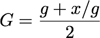
One way to calculate square roots is by using Newton’s method of successive approximations. We start with a guess g for the square root of a number x and calculate a better guess by averaging g with x/g, or:
The following procedure tests if the guess we have is good enough for the number x (the radicand) we want to compute the square root. If not it’ll keep trying to improve the guess until it’s good enough:
def sqrt_iter(guess, x):
    if is_good_enough(guess, x):
        return guess
    else:
        return sqrt_iter(improve(guess, x), x)
To improve a guess we average it by the number x divided by the guess:
def improve(guess, x):
    return average(guess, x/guess)
Average is easy enough to define:
def average(x, y):
    return (x + y)/2
Of course, we need to define is_good_enough. A basic test is to see if the
square of the guess minus the original number x is smaller than some threshold
(we use 0.001). This is not a good test for very small and large numbers (see
exercise 1.7 in the book) but will do for a first try:
def is_good_enough(guess, x):
    return abs(square(guess) - x) < 0.001
Finally, we need to start at some point. We begin with 1.0 as a guess:
def sqrt(x):
    return sqrt_iter(1.0, x)
Procedures as Abstractions
One problem with our implementation of sqrt is that functions like
is_good_enough, sqrt_iter and improve are cluttering the global namespace.
It’s very important to decompose a problem in sub-parts like we did, were each
function does only one thing, but it’s also important to be able to group things
that are not going to be used in other contexts (like improve and
sqrt_iter). One solution is to nest the procedures in one block structure:
def sqrt(x):
    def is_good_enough(guess, x):
        return abs(square(guess) - x) < 0.001

    def improve(guess, x):
        return average(guess, x/guess)

    def sqrt_iter(guess, x):
        if is_good_enough(guess, x):
            return guess
        else:
            return sqrt_iter(improve(guess, x), x)

    return sqrt_iter(1.0, x)
Now the functions sqrt_iter, is_good_enough, and improve are internal to sqrt and are not exposed to other programmers.
But there’s something else. The variable x is bound in the scope of sqrt and
since improve, is_good_enough, and sqrt_iter are in the scope of sqrt we
don’t need to pass x explicitly as as argument to these functions. We can
rewrite the code to make x a free variable inside these functions. In this
case the interpreter will get the value of x from the enclosing scope_._ This
is an example of lexical scoping:
def sqrt(x):
    def is_good_enough(guess):
        return abs(square(guess) - x) < 0.001

    def improve(guess):
        return average(guess, x/guess)

    def sqrt_iter(guess):
        if is_good_enough(guess):
            return guess
        else:
            return sqrt_iter(improve(guess))

    return sqrt_iter(1.0)
Summary
In the first section of SICP the authors introduce the notion of the environment and lexical scoping (both will be explored in more detail latter in the book), evaluation methods, and, above all, functional abstraction. I think this is a pretty sophisticated introduction for beginners and shows why SICP is considered one of the classics of computer science.